Surveyor SRV-1 Trail

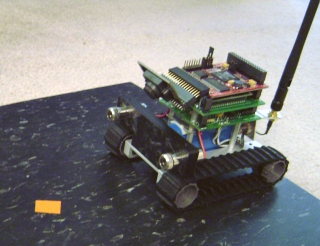
The Surveyor SRV-1b is a great platform for experimenting in machine vision. With the wireless communication and built in camera the SRV-1b is a natural choice for machine vision processing using a PC.

In this tutorial we once again experiment with object tracking. In this case we are looking for orange squares that define a trail for the robot the follow. The trial of squares is created using orange electrical tape cut in small pieces and placed approximately 1.5 inches apart. Care needs to be taken to place each square near enough to the previous square otherwise the robot will not be able to see the next square as it looses track of the previous one. Once the robot determines that no additional squares are present it will turn around and proceed back over the course.

The camera angle of the SRV-1b is more or less parallel with the floor. In order for this tutorial to work correctly the camera needs to be tilted down such that more of the floor is in view. This hardware adjustment is necessary otherwise the squares appear more like orange lines due to the large perspective distortion in the default view. The tilting of the camera was accomplished by using a 32 pin connector that fits into the camera socket and bending the pins using a vice to the desired angle. While this is not the most elegant solution it certainly worked for our purposes.

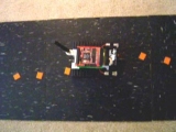
First left us have a look at our sample trail.

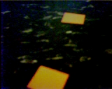
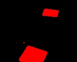
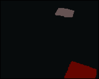
Sample Trail

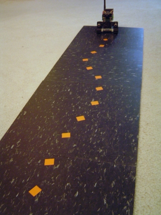
The image above is an overhead shot of the sample trail creating using orange electrical tape placed on black tiles. From an overhead view the contrast is very good with the squares being nicely defined against the matt black tiles.

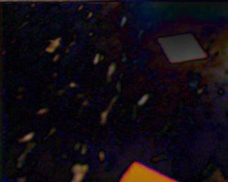
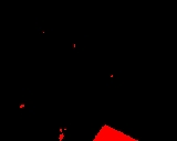
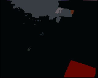
From the robot's point of view the setup looks quite different than from an overhead view. This is largely due to the proximity of the camera to the ground and the lack of adequate lighting to provide enough contrast in the image. The bad lighting of the setup was done on purpose in order to review image processing techniques that can help in these kinds of environments.

The robot view also reveals the pattern in the black tiles that includes white marks. These are less apparent in the overhead view but provide a high level of noise in the robot view.

You may also note that the squares in the image do not appear orange but instead appear more of a yellow color. This is due to color consistency problems which cause colors to appear incorrectly due to camera intrinsics, bad/low lighting and different illumination colors, i.e. colors appear different in sunlight versus florescent lights even if well lit.

Let's have a look at a couple more images from the robot..

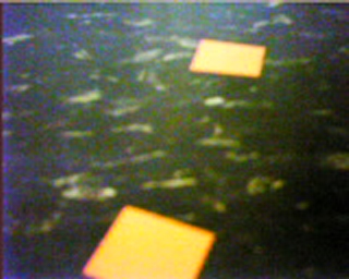
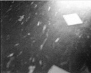
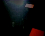
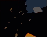
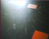
Robot View

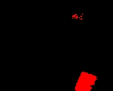
It turns out that the previous robot image view was in fact one of the better images! Things just get worse from that! The above image shows a capture from the robot's point of view on its way back over the course. Our setup is placed not far from an outside window. With the strong sunlight (we're in sunny Los Angeles, CA) the glare from the outside causes significant reflection on the black tiles. Despite being black the tiles appear white when in the appropriate reflective angle with respect to the outside light. Again, this bad lighting was done on purpose in order to review possible solutions to this environmental difficulty when you cannot change the environment. If you can change the environment then is always recommended that you do so, i.e. close the curtains!

You can also see from the above image that the "orange" square also suffers the same affliction as the black tiles. The upper square is actually orange but in fact appears completely white in this view due to the reflected light.

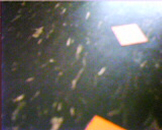
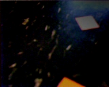
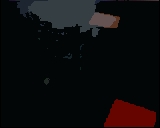
The final robot image view is also taken from the reflected sunlight angle but in this case the lower square finally reveals its true orange color. Yet in the very same image the upper square again appears white.

If you are new to image processing and machine vision you will by now start to gain an awareness of the importance of lighting in these scenarios. Lighting is a fundamental issue when working with robotic vision.

Given these three test images let's begin processing them in order to segment the squares from the rest of the image.

Lighting

We begin the orange square segmentation problem by working on the lighting issue. From the latter two robot images it is clear that the glare needs to be reduced.

A quick technique to resolve lighting issues is to reduce the image to edges. Most edge detection techniques use the local neighborhood of pixels in order to generate the edge strength. This local neighborhood has the advantage of reducing global lighting issues. This technique was used in one of our very first tutorials on line following. The technique requires edge detection and thresholding followed by detection of the Center of Gravity to determine the robot direction.

We can clearly see that while this technique does have some promise the edges detected also include edges from the white spots embedded in the black tiles. If you are using a surface that does not have these noise elements then edge detection is a possible way to go.

In the case of our trail following robot there is a problem at the end of the course when the robot turns around. During the turn proceedure the robot will momentarily see the tile edge against a lighter carpet. This boundary appears as a very strong edge which will cause the Center of Gravity measure to veer the robot off course.

Instead, we will try another light adjusting technique.

Lighting #2

We now proceed with a common lighting technique that will level the intensity of all pixels within an image. We will use one of the images to illustrate the process.

First, we convert the image to grayscale using the Grayscale module. This essentially focuses the image into its luminance or lighting channel. This is the channel that we want to even out within the image.

Next we really REALLY blur the grayscale image using the Mean module.

From this blurred image we subtract the original color image using the Math module.

Which results in a much more even intensity across the entire image. This technique works because the grayscale conversion focuses on the intensity channel, the blurring relaxes the edges caused by lighting to effect large areas and the subtraction removes the global lighting changes to leave just the localized intensity changes which are typically associated with edges. This is in effect a form of an edge detector but one that better preserves the image colors than most edge detection techniques.

Now let's try detecting colors.

Colors

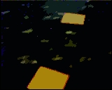
In order to detect the squares we need to identify them from within the image. Lets try using colors to detect them. Let us review what the three test images currently look like now with more even lighting.

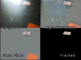
Using the RGB_Filter module to search for red (yellow and orange both contain red) reveals some interesting but incorrect results.

The first image seems fine but the last two mostly miss the upper square. If this happens during the course the robot will start turning around prematurely as it will think that the course has come to an end.

As in apparent from the above images using color to detect a gray object is not going to be very fruitful. In this case we now abandon color as an identification feature and use it more as a natural pixel grouping feature.

Flood Fill

As we can no longer rely on color as a tracking feature we now turn to shape. To extract objects based on shape we first need to ensure that the object can be analyzed as an object. This means we need to group similar colored pixels with each other to define an object or a blob as known in machine vision terms.

Using the Flood_Fill module (set to 65) we apply a color flattening technique to merge pixels into more meaningful groups. Flood filling is similar to the flood fill that is present in most paint programs. If a pixel is of similar color to its immediate neighbor the two pixels are replaced with the mean color of the two.

This works well to define objects but we still have a problem with image #3. If you look closely the upper square is almost a single color but has a large part of it on the right hand side in another color. This is caused by the tolerance of the flood fill not being high enough to include that part of the blob as a single object. However, increasing the tolerance causes other undesirable effects such as merging the square into the background glare.

Instead we use another feature of the Flood Fill to analyze neighboring blobs and how intense their borders are. The original edge detection tests showed that the outline of the squares were the only dominant edge in each square. The border between the parts of the upper square blob in image #3 above is then not very significant. Thus we use the Merge Borders interface in the flood fill to help merge blobs whose borders are not very strong.

This also has the added benefit of merging the glare objects into a single background blob further decreasing the image noise. Now that we have all of our squares a single color we can start analyzing the shapes of the remaining blobs.

Blob Filter

To extract only the square shapes from the image we utilize the blob filter and the Quadrilateral Area to quantify the resemblence of the blob to a square. The Quadrilateral Area attribute analyses the sides and area of each of the blobs to calculate how close the blob area is to a quadrilateral defined by the 4 major sides of the blob. I.e. how well does the blob fit into the concept of squareness.

The blob filter allows you to add in descriptive attributes that rank each of the individual blobs according to the feature they represent. Thus, for a perfect square we would expect a rank of 1.0 whereas for blobs that are less square we would expect a <1.0 weight.

Reviewing our test images shows that a cutoff value of around 0.65 would segment all our actual squares from the rest of the detected blobs. The other detected blobs are artifacts from the tile's white spots and the sunlight glare that we reduced earlier on.

If is worth noting that the squares on the sides of the images may or may not be detected by the square shape as part of the square is cutoff from the image. This is not an issue as we also use the blob filter to remove any blobs that touch the border. The reasoning is that we know all squares will fit into the image view and anything on the sides will either come into view or if just going out of view. We also remove border objects as the robot when moving may cause previously seen blobs to once again be detected. This detection can cause the robot to occilate back and forth as the object moves in and out of partial view of the camera.

Using a 0.65 threshold and adding the COG module ends our image processing process as we now have an approximate point (the COG) for the robot to follow. The red circle identifies the COG point.

Note that if more than one square is visible on the screen the COG will return a average point between the two squares which is desirable as it evens out the transition from one square to the next.

Now that we have the point to move towards we need to use that information to control the SRV-1b appropriately.

VBScript

The point we want the robot to move towards is contained in the COG_X and COG_Y variables. These variables are created by the Center of Gravity module.

To control the motors of the SRV-1b to move towards that point we need to just use the X coordinate and steer left if the point is to the left of the screen or right if the point is towards the right of the screen. Basically we want to control the robot to keep the X COG in the middle of the screen. This will then cause the robot to move along the defined trail and also attempts to keep as much of the significant part of the image (i.e. the squares) in view.

We use the VBScript module to create two motor variables that are then fed to the Surveyor SRV-1b module.

Surveyor SRV-1 Trail Video

(1.5 MB) Video of the SRV-1b as it makes its way along the trail. You can see each of the major steps along the way as the image is processed for lighting, flood fill and blob filtering.

(1.7 MB) Overhead video of the robot moving along the trail.

(1.3 MB) Standalone video of what the robot sees while moving along the trail for your own testing purposes.

Problems

It is worth pointing out some of the issues and mistakes that we experienced during the creating of this tutorial to help you solve similar issues.

1. Lighting - To illustrate different lighting techniques we purposely made the setup environment non-optimal to run the robot. In reality one would probably attempt as much as possible to ensure that the lighting requirements are better met and no sunlight glare is present. This could also have been better mitigated by using different tiles that reflect less light.

2. Blob-Filter - Removing blobs based on attribute values is somewhat of a black art. As with any image processing applications noise is ever present in the image and can cause some of the squares to become non-square's momentarily. This causes them to disappear from the robots tracking. Better flood filling and blob filtering might be able to reduce this loss of tracking seen as object flicker in the final videos.

3. Motion blur - Capturing images while the robot is moving causes motion blur in the captured image. This motion blur tends to cause the squares to become more irregular in shape and therefore not match the blob filter criteria. To reduce the effects of motion blur the robot is pulsed in-between image captures to ensure that the robot is not moving while an image is being captured. This does slow down the robot movement considerably but is a necessary requirement for stable operation.

4. Frame rate - Despite the SRV-1b being capable of more than 10fps when in 160x128 mode the low/bad lighting further reduces the processed frame rate to less than 4fps. This reduction also requires that the robot move slower in order to capture enough frames to react quickly enough to steer the robot. The pulsing added to reduce motion blur provided enough speed reduction to ensure that the robot could react to the visual scene fast enough.

5. Oscillation - There are still times where the robot has successfully passed a square but during the turn (due to the robot being a tracked vehicle) the robot may back up enough to again see the most recently passed square. This causes the turn to terminate and the robot to reengage tracking. Once passed, the robot returns to turning mode where the process can repeat itself. This issue can be reduced by further increasing the time after which the robot determines it is no longer seeing a square and when to start a turn execution. Addition filters can also be added to eliminate detection of any square in the lower part of the image while turning with the assumption that any square that should now be tracked would appear somewhat distant from the robot.

Your turn ...

Want to try this yourself?  Download the Surveyor SRV1b Trail robofile that you can run yourself. Clicking on any of the modules will bring up that interface and allow you to customize it for yourself.

The End

That's all folks. We hope you've enjoyed this little adventure into an application of machine vision processing. If you have any questions or comments about this tutorial please feel free to contact us.

Have a nice day!

New Post

Surveyor SRV1b Trail Related Forum Posts	Last post	Posts	Views
None