
Visual Line Following
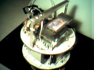
The following tutorial is one way to use a vision system to identify and follow a line.The system uses:
- single CCD camera
- USB Digitizer
- Pentium CPU on board
- Left, Right differential motors
Example Images
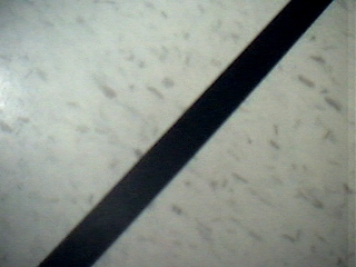
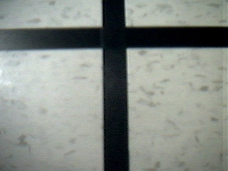
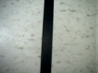
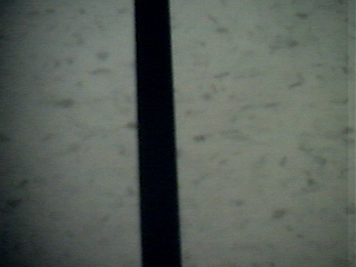
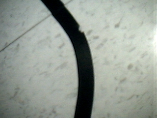
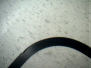
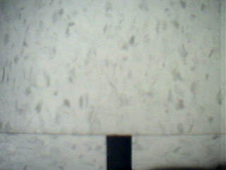
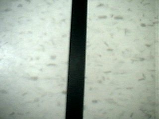
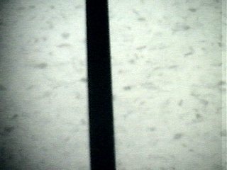
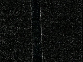
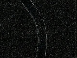
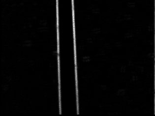
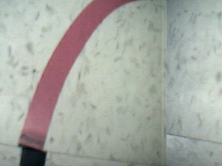
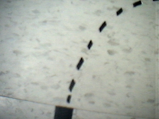
To get a better idea of what we're trying to accomplish lets first look at some sample pictures that the BucketBot took. The images are from the CCD camera mounted to the front of the BucketBot angled towards the ground.Note that we have not done any calibration of lighting adjustments. The images are straight from the camera.
If it worth mentioning that the lines are created by black electrical tape stuck on moveable floor tiles. This allows us to move the tiles around and experiment with shapes quite easily.
Lighting Issues...
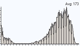
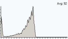
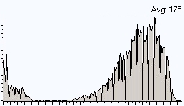
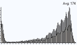
Bad lighting can really cause problems with most image analysis techniques (esp. when thresholding). Imagine if a robot were to suddenly move under a shadow and lose all control! The best vision techniques try to be more robust to lighting changes.To understand some of those issues lets look at two histograms from a straight line image from the previous slide. Next to each of these images are the images histogram. The histogram of an image is a graphical representation of the count of different pixel intensities in the image.
As you can see, histograms for lighter images slump towards the right (towards the 255 or highest value) whereas darker images have histograms with most pixels closer to zero. This is obvious but using the histogram representation we can better understand how transformations to the image change the underlying pixels.
The next step is to see if we can correct these two images so that they look closer to one another. We do that by normalizing the images.
Normalize Intensities
To counter the effects of bad lighting we have to normalize the image. Image normalization attempts to spread the pixel intensities over the entire range of intensities. Thus if you have a very dark image the resulting normalization process will replace many of the dark pixels with lighter pixels while keeping the relative positions the same, i.e. two pixels may be made lighter but the darker of the two will still be darker relative to the second pixel.By evenly distributing the image intensities other image processing functions like thresholding which are based on a single cutoff pixel intensity become less sensitive to lighting.
For example, the following images from the previous page show what happens during normalization. It is important to note that any image transformation that is meant to improve bad images must also preserve already good ones. In testing image processing functions be sure to always understand the negative side effects that any function can have.
Normalization did not create much change because image was lighted ok to begin with.
The bad image experienced a large amount of change as the image intensities did not cover the entire intensity range due to bad lighting. You can see from the histogram that the image intensities are now more evenly distributed.
Also you can note how the new histogram appears to be not as solid as the original. This is due to how the intensity values are stretched. Since the new image has exactly the same number of pixels as the old image the new image still has many pixels intensity values that do not exist and therefore show up as gaps in the histogram. Adding another filter like a mean blur would cause the histogram to become more solid again as the gaps would be filled due to smoothing of the image.
Next we need to start focusing on extracting the actual lines in the images.
Edge Detection
In order to follow the line we need to extract properties from the image that we can use to steer the robot in the right direction. The next step is to identify or highlight the line with respect to the rest of the image. We can do this by detecting the transition from background tile to the line and then from the line to the background tile. This detection routine is known as edge detection.The way we perform edge detection is to run the image through a convolution filter that is 'focused' on detecting line edges. A convolution filter is a matrix of numbers that specify values that are to be multiplied, added and then divided from the image pixels to create the resulting pixel value.
To learn more about convolution filters have a look at our help section.
We will start with the following convolution matrix that is geared to detect edges:
| -1 | -1 | -1 |
| -1 | 8 | -1 |
| -1 | -1 | -1 |
The next step is to run the images through this edge detector and see what we get ...
Edge Detection
Here are two sample images with the convolution edge detection matrix run after normalization:
It is interesting to note that while the convolution filter does identify the line it also picks up on a lot of speckles that are not really desired as it causes noise in the resulting image.
Also note that the detected lines are quite faint and sometimes even broken. This is largely due to the small (3x3) neighborhood that the convolution filter looks at. It is easy to see a very large difference between the line and the tile from a global point of view (as how you and I look at the images) but from the image pixel point of view it is not as easy. To get a better result we need to perform some modifications to our current operations.
Modified Line Detection
To better highlight the line we are going to:1. Use a larger filter; instead of a 3x3 neighborhood we will use a 5x5. This will result in larger values for edges that are "thicker". We will use the following matrix:
| -1 | -1 | -1 | -1 | -1 |
| -1 | 0 | 0 | 0 | -1 |
| -1 | 0 | 16 | 0 | -1 |
| -1 | 0 | 0 | 0 | -1 |
| -1 | -1 | -1 | -1 | -1 |
2. Further reduce the speckling issue we will square the resulting pixel value. This causes larger values to become larger but smaller values to remain small. The result is then normalized to fit into the 0-255 pixel value range.
3. Threshold the final image by removing any pixels lower than a 40 intensity value.
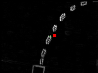
The results of this modified technique:
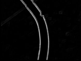
We now nicely see the line edges and most of the noise speckles are gone. We can now continue to the next step which is how to understand these images in order to map the results to left and right motor pulses.
Center of Gravity
There are many ways we could translate the resulting image intensities into right and left motor movements. A simple way would be to add up all the pixel values of the left side of the image and compare the result to the right side. Based on which is more the robot would move towards that side.At this point, however, we will use the COG or Center of Gravity of the image to help guide our robot.
The COG of an object is the location where one could balance the object using just one finger. In image terms it is where one would balance all the white pixels at a single spot. The COG is quick and easy to calculate and will change based on the object's shape or position in an image.
To calculate the COG of an image add all the x,y locations of non-black pixels and divide by the number of pixels counted. The resulting two numbers (one for x and the other for y) is the COG location.
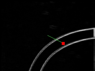
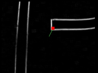
The COG location is the red square with a green line from the center of the image to the COG location.
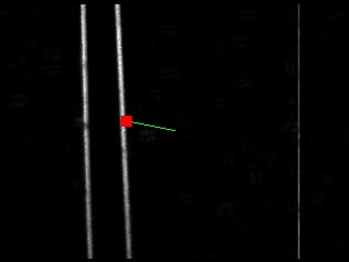
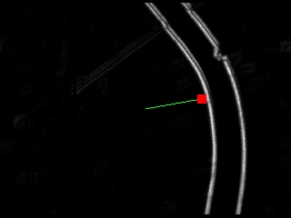
Based on the location of the COG we can now apply the following conditions to the robot motors:
- When the COG is to the right of the center of screen, turn on the left motor for a bit.
- When the COG is on the left, turn on the right motor.
- When the COG is below center, apply reverse power to opposite motor to pivot the robot.
You can also try other conditions such as when the distance of the COG to the center of screen is large really turn up the motor values to try to catch up to the line.
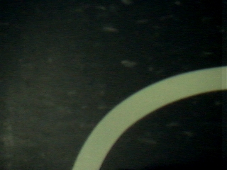
This technique works regardless of the color of the line ... as long as the line can be well differentiated from the background we can detect it!
It even works if we reverse the original black line on white tile assumption.
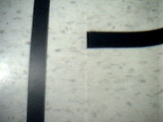
In fact, we don't really even need a connected line!
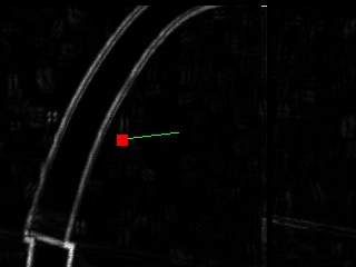
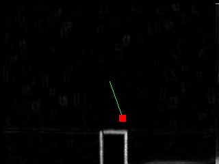
Here is a case where the end of the line is reached. Notice that the COG has fallen below the center of the screen. Perhaps we can use this condition to stop the robot!
Opps, a mistake! The robot will start following the wrong line ... but there again no technique is perfect.
Your turn ...
Want to try this yourself? Following is the robofile that should launch RoboRealm with the original image we used in this tutorial. You can click on each of the steps in the pipeline to review what the processing looks like up to that point.
![]() Download Line following .robo file
Download Line following .robo file
The End
That's all folks. We hope you've enjoyed this little adventure into an application of machine vision processing. If you have any questions or comments about this tutorial please feel free to contact us.
Have a nice day!
| New Post |
| Line Following Related Forum Posts | Last post | Posts | Views |

hi steven I see the tutorial but I don't understand some function. if i want to chec... |
11 year | 12 | 5175 |
|
LINE FOLLOWING
HI, STEVEN I DON'T UNDERSTAND SOME VBScript x = GetVariable("COG_X") y = GetVariable("... |
11 year | 1 | 3678 |
|
visual line folllowing
HI steven, i don't understand the function in VBScript x = GetVariable("COG_X") y = Ge... |
11 year | 1 | 3692 |
|
RR for Line tracking
Hi, I am new to these ROBO world.I want to experiment on building a ROBOT which can follow the track using USB Camera mounted on... |
12 year | 2 | 4236 |